
This short write up is essentially about the idea that when people want to get rid of cheaper currencies in their wallets, these currencies tend to take up a larger portion of all currencies currently in use.
What we could expect is that these “bad currencies” will finally settle and fall into the wallets of those people, to which these “bad currencies” are home currencies - since they will use them more often then foreigners.
This turns out to be not that obvious - maybe because of statistical variance in the simulation or the generalistic assumptions I used. Or maybe this is simply not the case, and Copernicus was right in a much more broader sense.
I also looked at some retail movie data and observe that similar to “bad currencies”, “bad movies” also outperform the “good movies”.
Intro
In September 2023 Polish Central Bank created a high school competition for an essay in economics exploring the persona of a XVI century astronomer Nicolaus Copernicus.
 Nicolaus Copenicus (1473-1543)
Having learned about it 10 days before the deadline, discarding my other schoolwork, I have managed to upload a rough version of my exploration. The main part of the essay, which I think is pretty interesting, is a simple model of a multi-currency market I will describe in this post. Project repository is under this link.
Copernicus-Gresham’s law
Copernicus law has been mistakingly attributed to a scottish economist Thomas Gresham, due to a recurring error of works following the infamous Henry Dunning Macleod’s study The Theory of Credit. It was actually first consistently described in Copernicus’ Monete Cudende Ratio. (Source)
The law is a monetary principle stating that “bad money drives out good”. For example, if there are two forms of commodity money in circulation, which are accepted by law as having similar face value, the more valuable commodity will gradually disappear from circulation. (definition from Wikipedia page)
In Monete Cudende Ratio Copernicus also highlights the high possibility of loss of the country, as - based on historical facts he remarkably analyzed - foreign traders had demanded payments in the better version of a coin (the one containing more silver.)
The model
In short, the model is about agents who perform transactions (transfers of funds) in a particular currency.
If you don’t care about the details, skip to the Simulation results part.
Simulation process
The environment is first initialized with arguments given in this Python command: (see project repo)
1
2
3
4
5
6
7
8
9
10
11
12
13
14
15
python \.simulate.py --population_size 1000
                     --number_of_countries 4
                     --number_of_currencies 4
                     --even_countries_currencies_spread True
                     --number_of_transactions 100
                     --number_of_episodes 500
                     --figure_convolution_window_size 10
                     --save_figure False
                     --verbose True
                     --alpha 20
                     --beta 0.5
                     --gamma 0.0086
                     --delta 1.5
                     --epsilon 0.5
                     --zeta 10
Then, over the course of all episodes, randomly chosen agents perform a series of transactions between one another.
Initialization
At this stage each country gets an assigned home currency. Each agent gets an assigned country id (chosen randomly from a uniform distribution) and a wallet of currencies, which is a list of numbers (same size for every agent) chosen uniformly from the interval $[0, 1]$. Agent’s home currency value is then multiplied by a parameter alpha $>1$ as to imitate realism - it’s natural to think that people/firms have more funds in their home currency for everyday expenses/overhead costs.
Currency exchange in the current model version is constant and is hardcoded into the model to be of currencies: USD, EUR, CHF and GBP.
Note: to simplify experimental analysis there is a parameter
even_countries_currencies_spreadthat ensures currency assignment to countries is not pure random, but spread evenly.
Transaction
When a transaction begins, we first choose one random agent from the population, call him buyer. To choose the seller (receiver of funds) we first assign probabilities to countries, so that an agent from buyer’s home country is gamma times more likely to be chosen.
With buyer and seller established, we choose the transaction value (as of now measured in the primary currency.)
Note: primary currency in which all calculations are done is currency with index 0 - it’s assumed this way for the sake of simplicity
Transaction value, call it $\texttt{t}$ is uniformly chosen at random from the interval $[0, \texttt{budget} \times \texttt{beta} ]$ where $\texttt{budget}$ is buyer’s total wallet value in the primary currency. We interpret beta as the maximum fraction of his total budget an agent is willing to spend.
Next we iterate through buyer’s wallet and see what currencies have sufficient funds (that is their value in primary currency is $\geq \texttt{t}$) to record them in some list $\texttt{valid-currencies}$.
Then we iterate through $\texttt{valid-currencies}$ and assign special values to these valid currencies to store them in an array $\texttt{perceived-values}$.
To understand what is going to happen, consider this short example.
Example:
Imagine the buyer’s wallet is \([\$10, \text{£} 15 ]\), his as well as seller’s home currency is \(\$\) and the exchange is \(\$ 1 = \text{£} 0.82\) (so \(\$ 1.22 = \text{£} 1\). ) The buyer has chosen the transaction value to be \(\$5\) (but has not chosen the currency yet.)
We can assume a couple of (crucial) things:
- buyer is more likely to make a transaction in his home currency if the seller is from his own country;
- due to Copernicus’ work, it is natural to think:
- that the lower the currency value is, the more likely the buyer is to want to get rid of it and therefore to use it in the transaction
- following the previous point, the less primary value the buyer has in this currency (in his wallet), the more likely he is going to use it
In the above scenario we might think that since the dollar is \(1.22\) times less expensive, the buyer should be \(1.22\) times more likely to use it. . Moreover, since he has much less primary value (\(\$ 10\)) in dollars compared to pounds (\(\text{£} 15 = \$ 18.26\)) he should be \(18.26 / 10 = 1.826\) times more likely to use the dollar. In fact, considering that the home currency of both the seller and the buyer is USD, the likelihood of choosing it gets multiplied by some constant zeta \(> 1\) (zeta was assumed to equal \(10\) in many simulations.) Ultimately, when the buyer makes his mind, we expect the probability of choosing the dollar be \(1.22 \cdot 1.826 \cdot 10 = 22.2772\) times more likely.
What is calculated in the model, are temporary scores of each option (currency) which are then used to be inversely proportional to probabilities of choosing a currency (the higher the score the lower the probability.) The decision mechanism was based on the idea described in this post.
So in our example the temporary score of the dollar (given delta = 1.5, epsilon = 0.5) is:
and of the pound:
\[1.22 ^ {1.5} \cdot 18.26 ^ {0.5} \approx 5.758\](Note we didn’t divide the pound by zeta since it is not both buyer’s and seller’s currency at once. In this subexample we also assumed different values for delta and epsilon: you should convice yourself they were previously assumed to be both $1$.)
Hence based on the mentioned probability mechanism the likelihoods of the chosen currency $C$ being the dollar/pound are:
\[P(C = \$) \approx \frac{\frac{1}{0.316}}{\frac{1}{0.316} + \frac{1}{5.758}} \approx 0.948\] \[P(C = \text{£}) \approx \frac{\frac{1}{5.758}}{\frac{1}{0.316} + \frac{1}{5.758}} \approx 0.052\]Going back to the simulation: the perceived values (temporary scores) of each currency \(C_i\) are
\[\text{Primary value of $C_i$} ^ \texttt{delta} \times \text{Primary value of buyer's wallet in $C_i$} ^ \texttt{epsilon}\]in case it is a home currency of both the buyer and the seller, we divide it by zeta.
Next, we plug in these temporary scores to the probability mechanism and use the resulting probabilities to randomly choose the currency in which the transaction will be taken.
Next we transfer the funds, so simply subtract the value of buyer’s wallet at the chosen currency wallet index and add it to the appropriate index of the seller.
Parameters summary
| Parameter | Type | Explanation |
|---|---|---|
| –population_size | int | |
| –number_of_countries | int | |
| –number_of_currencies | int | Has to be smaller or equal to the number of countries |
| –number_of_transactions | int | |
| –number_of_episodes | int | |
| –figure_convolution_window_size | int | With how many values do you average out curve |
| –increase_weakest_currency | bool | Whether to increase the weakest currency over all the episodes |
| –even_countries_currency_spread | bool | Whether there should be an evenly distributed spread of assigned currencies between countries |
| –save_figure | bool | |
| –verbose | bool | Whether to log progress of the simulation |
| –alpha | float | How much more money is an agent expected to have in his home currency |
| –beta | float | What maximum percent of his budget is an agent willing to use for a transaction |
| –gamma | float | How much more likely is an agent to make a transaction with someone from their own country |
| –delta | float | How much more impact on the probability of choosing currencies does their value have |
| –epsilon | float | How much impact on the probability of choosing currencies does agent’s wallet contents have |
| –zeta | float | how much impact on the probability of choosing currencies does the fact that the seller is from the same country has |
Simulation results
To gain insight on the simulation process we need to collect some data. In particular, it would be useful to track what proportion of transactions are those with a higher primary value - as to explore the extent to which Copernicus Law holds.
The model collects data about two things:
Total transaction value in a currency over time. Every episode we record data on what currencies people used and in what quantities. These are then plotted on the top figure in the resulting image. For demonstration I also included a black line that describes how far does an episode deviate from a scenario, in which total transaction values are ordered inversely to their exchange rate value (the cheaper it is the more it is used.)
Total transaction value in between different countries over all episodes. Every episode we record data on what currencies people used and in what quantities to record it in an aggregated list of matrices. Each currency has one relationship matrix that describes how much transaction in this currency happened between pairs of countries.
Below is an example simulation result with above mentioned features. In the first case, I have gradually increased the value of the cheapest currency to become slightly more expensive then all others. In the second, I did not.
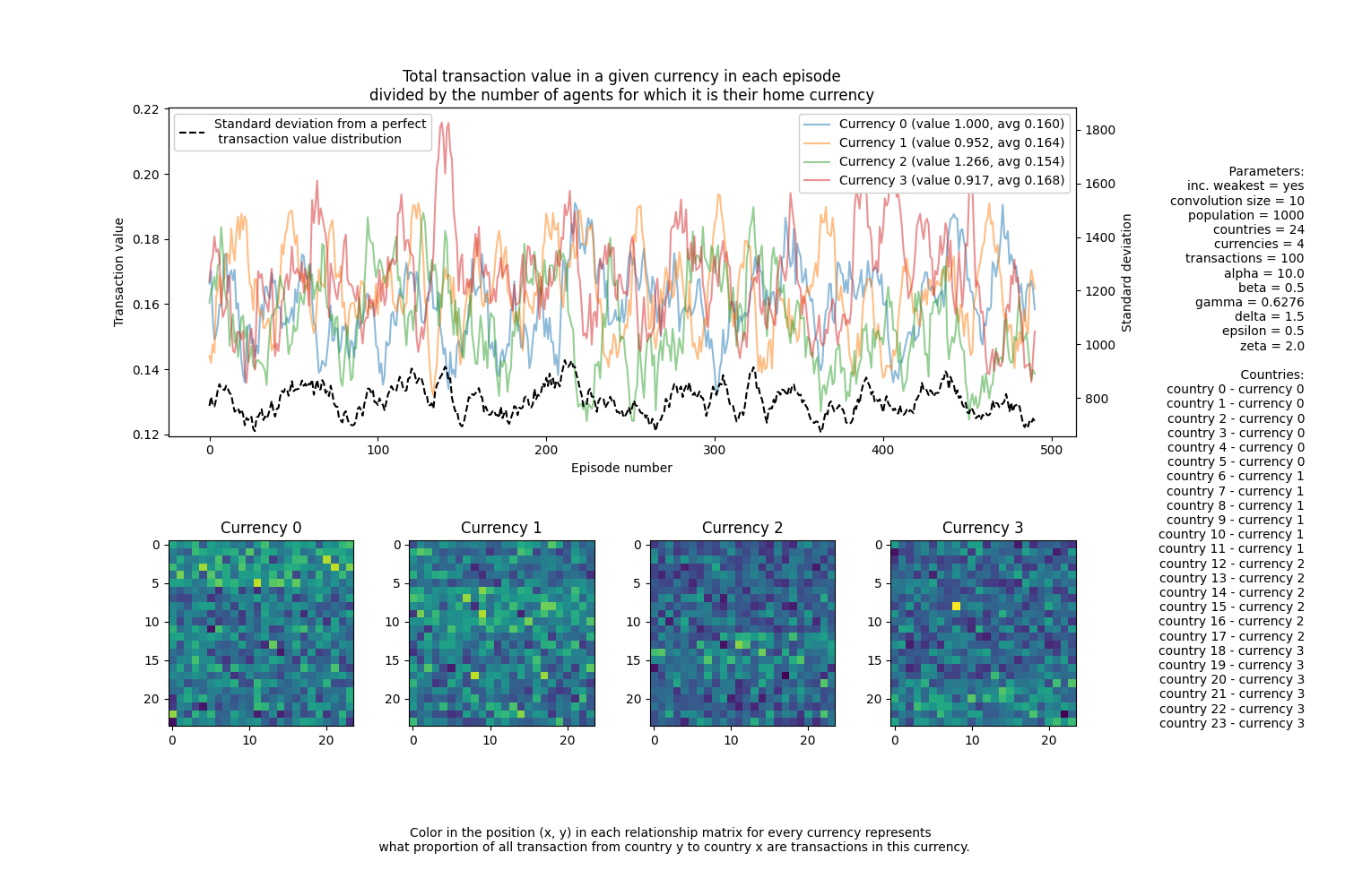 Gradual increase
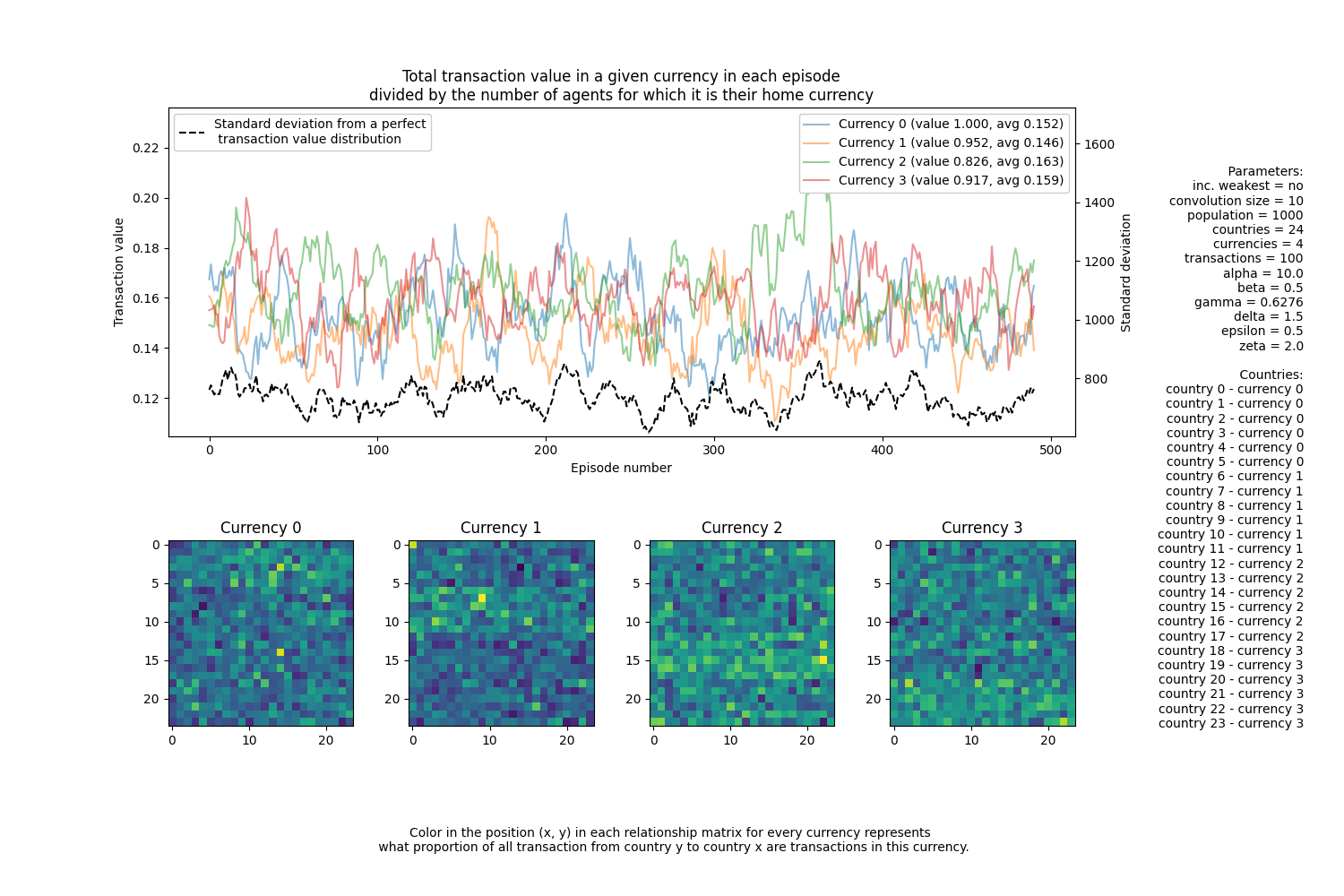 No gradual increase
I encourage the reader to play around with the model’s parameters and see what happens. Because there are so many of them to tweak, this post would have been too large. I didn’t include all possible combinations. You can only trust me that the same pattern holds.
The primary thing we can observe is that the cheapest currency has the highest usage frequency: on both graphs, their average total value (avg) is the largest. What is really interesting, is that even in the second case (as we tweak the whole exchange rate) the cheapest currency also begins to dominate the circulation!
Note: in the graph,
avgreally stands for the average value of transactions measured in the home currency. It is also normalized by the number of people in each country. So the above observation are perhaps not as strong as they may seem. But I would argue they are strong enough to consider the cheapest currency to “dominate”.
Investigating simulation results
The hypothesis I have described in the very beginning goes as follows: at some point we would expect the cheapest currency to fall out of the circulation. This would happen only if the total transaction value in the “bad currency” would not be a Mean reversive process. More precisely, at some point there would a significant change in the amount of “bad currency” being used. So the mean of the process would have changed - the time series wouldn’t have been stationary, exactly like in the bottom case.
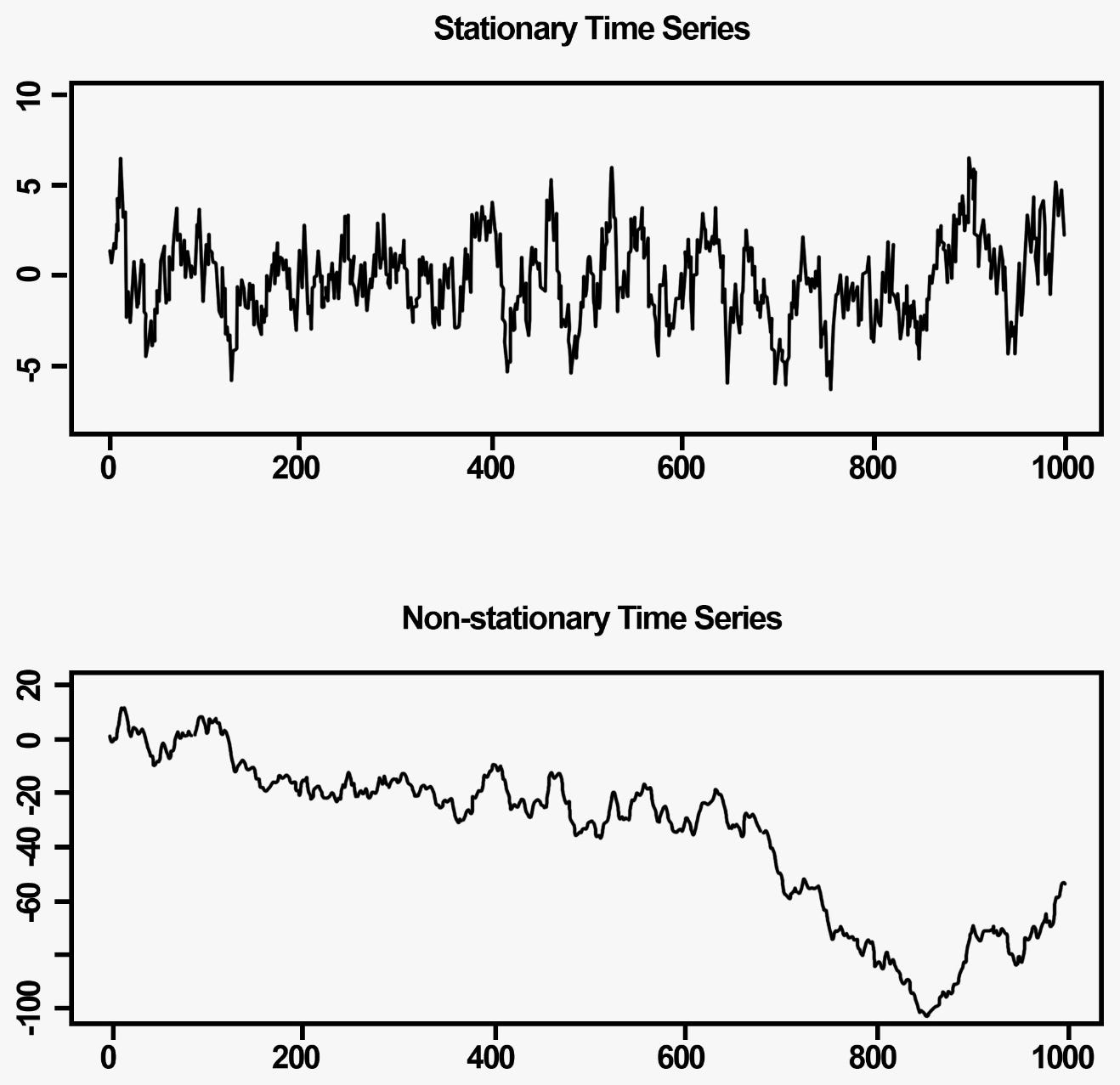
Although you can see on the previously shown experiment results that transaction values were stationary all along, I also run an additional ADF test in Python. It rejected the hypotheses that any of the processes were non-stationary. So they are stationary. They have a consistent mean and variance. You can check it yourself by running simulate.py.