
In September 2023 Warsaw Stock Exchange (WSE) hosted another edition of a high school trading competition, with the first stage spanning three months. I lead a 4 person team to implement a pairs trading strategy and research for others, including portfolio optimization. Repository for this project will be available under this link.
This is a description of what happened throughout, along with most of the technical details.
tldr; With neatly scraped data I implemented a Pairs Trading strategy, realized we aren’t able to short sell stocks, backtested it’s long-only version using an inverse ETF, got bad results, gambled all-in with Non-stationary Transformers and gambled all-in again with the most volatile stock on the market. Ultimately gained 2%, only to see all teams got admitted to the second stage.
SIGG game description
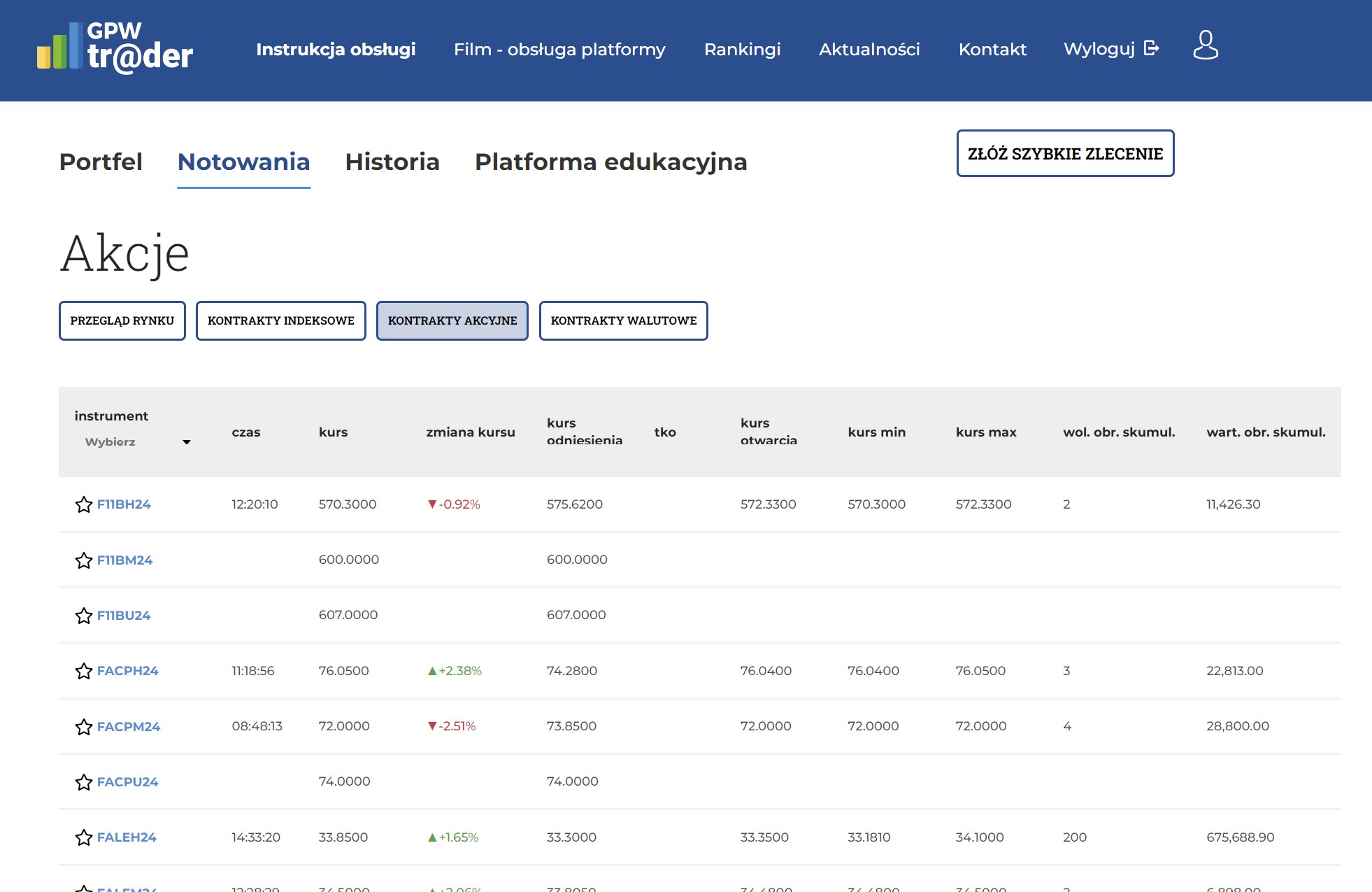
Out of all 381 stocks that are available on WSE the game offers 60, along with 11 ETFs and 3 WSE indices (WIG, WIG20, MWIG40.) Each team gets 20k PLN assigned.
The game offers orders of types: Market order, Limit order, Stop order or Stop limit order. We made only market orders, buying/selling at the currently traded market price.
The second stage additionally offered the use of Futures, which will hopefully be the topic of the next post.
Legal disclaimer
The game rules fortunately prohibited only the use of automatic trading systems - “computer software that enables automatic transaction execution is not allowed” (SIGG rules) - it did not explicitly mention an external analytics program we would make to suggest trades. These market orders of course would be ultimately made by us.
Data collection
With the incredible help of my friend Mikołaj WSE data was scraped and aggregated (for personal & educational purposes only!) from an API endpoint originally intended for graphical display of figures.
To filter out only the 74 assets from 381 available, I copied the SIGG webpage HTML code and parsed it through ChatGPT to obtain relevant Ticker names.
Strategies
The single most important thing we had in mind was that in order to gain any significant advantage over our competition, we shouldn’t be following the general market trend, i.e. buy the stocks strongly correlated with the Polish market index WIG20, as this is what the majority of people would perhaps do.
To get to any respectable position in the ranking, we should instead be trading the most volatile of stocks, following the market principle that the higher the risk, the higher reward.
It becomes apparent when we look at the data: in the previous years around 30 teams gained any sort of prizes, out of 10k studens (so about 4000 teams). The top team got a return of $17\%$ in half a year, which is pretty extraordinary - the baseline S&P500 index should return $11.36\%$ annually on average (which we have access to through the ETFSP500) so every six months the average investor would tend to earn $\sqrt{11.36\%}=3.37\%$, not $17\%$.
Still, this is a strategy we were willing to take only if our main approach would not work. And it didn’t.
Portfolio optimization
Based on the dataset provided, Wojciech Siostrzonek did research on the given stocks with PyPortfolioOpt.
From what we discussed with Wojciech, all considerable allocations contained the main market component. Therefore we speculated they would oscillate around the boring SP500 average, so we dropped this idea and proceeded further.
Pairs trading
In essence (and my understanding), the trading approach comes from the observation that some pairs of assets tend to be cointegrated; over time, their difference (or ratio) always comes back to some average value.
There are many caveats of course, like the average value majorly changing: for instance, when in a pair of two similar companies one’s Board of Directors would fire their founder CEO, a permanent divergence between their stock prices could appear.
When we find a cointegrated pair, we make profit by entering a long position on a stock that has diverged excessively downwards (we earn on it’s growth) and entering a short position on a stock that has diverged excessively upwards (we earn on it’s drop.) In case both stocks’ price change in the same direction (they both fall or rise) the profits on one of them compensate the losses on the other.
For more comprehensible reference, see this article or this Python notebook.
In our case, which spanned only 3 months, I considered only the prior 6 months to check for cointegration. If we were to consider much longer periods (like the past 2 years) we might have implicitly included events like COVID19, which might not have been so relevant in the current relationships between companies.
In case of the actual pairs trading, I first aimed to check the prior 3 months for finding the Z-Score trading signals (when to enter/exit the positions.) In the end it didn’t really matter since I didn’t have any opportunity to backtest this strategy, as I immediately began refactoring to the version without the ability to short.
Finding the pairs
We can deduce a pair of stocks is cointegrated if their difference is a stationary process - a time series that has a constant mean and variation. A statistical test to check if a process is stationary is already implemented in the SciPy library.
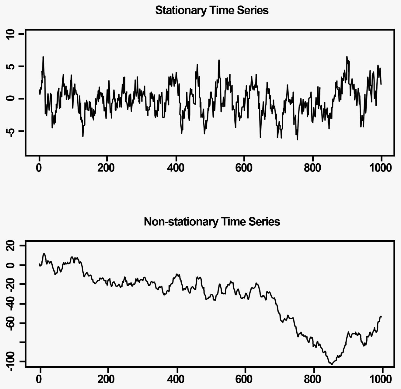
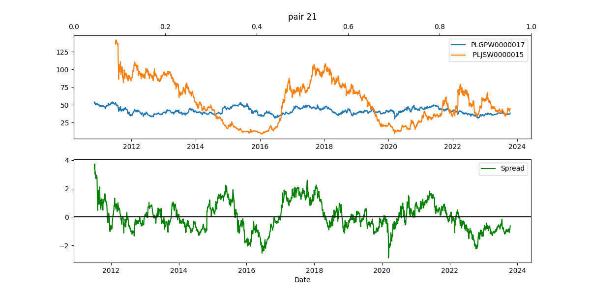
After iterating through the ${74 \choose 2} = 2701$ pairs, which took only a couple of seconds, I considered only the 1000 best pairs (ones most likely to be be cointegrated.) Next, I excluded many pairs through ranking the newly obtained pairs by the number of times the difference crossed the x-axis (see image below.)
In the end I manually inspected 172 pairs, excluding the ones which seemed to be cointegrated by an accident (like when a Software firm was paired with a Metalurgy industry firm.)
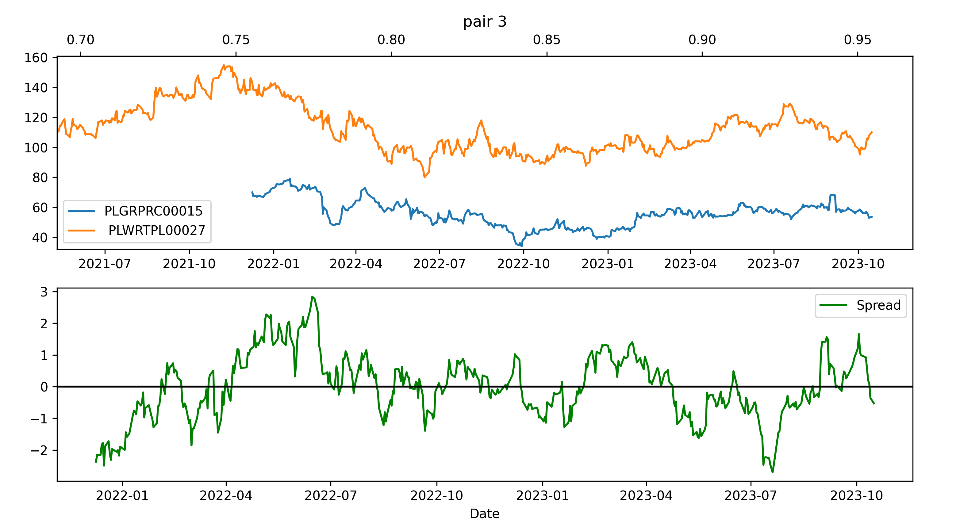
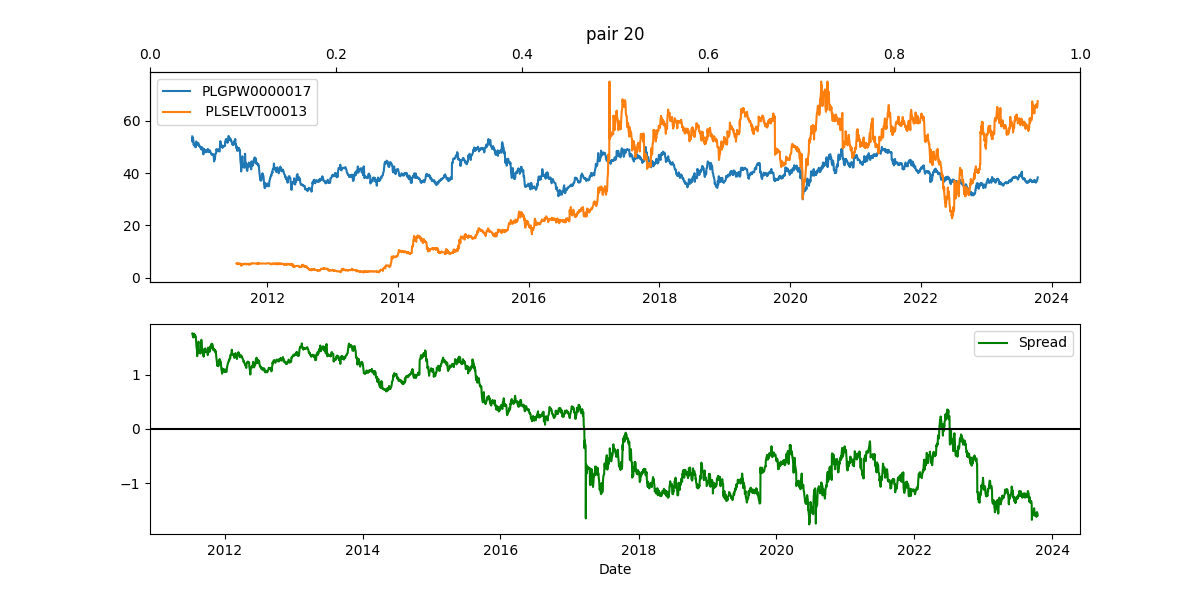
Moreover, it looked like many pairs were following the general market trend - they were paired with the Polish Market Index GPW; their high volatility induced a large number of crossings in the spread graph. Here are some examples, with the blue line displaying the GPW Index:
Ultimately we settled for 4 pairs of online services, 6 pairs of banks, 1 pair from the energy sector, 1 pair from the software development sector and 1 pair of an international firm and the polish market index.
Trading with the pairs & system overview
Now that we have chosen a list of pairs, our system keeps them in a file setup.csv. For each pair I have specified what portfolio percentage (out of all 20k PLN) will be employed. Additionally we keep track of previous stock prices in a database_2024-01-01_12:00.csv (updating the name with each content addition) and previous trades in trades.csv.
The deployed program goes through the following stages: first, it collects the newest price data. Next, it calculates our position based on trade history and analyzes whether the spread of each pair of stocks has increased/decreased since last time the spread was longed/shorted. Finally, it sends out emails to our team members with recommendations and charts.
The analysis of whether the spread is abnormally high or low can be done with various methods, including Kalman Filters or Deep Learning. Here, inspired by this post amongst others, it is simply performed by looking at the Z-Score based on the previous 3 months - if current Z-Score crosses a certain threshold (so e.g. it’s outside of $[-1.6, 1.6]$) and if we have sufficient funds, then we enter an appropriate position. If we had an open position earlier and the Z-Score fallen into some safety range (e.g. $[-0.5, 0.5]$), then we exit the entire position on this pair.
Note: in this context (and internal repository documentation) it is assumed that longing the spread means longing the first stock in the pair and shorting the other, as it is ordered in
setup.csv
More specifically, finding the signal boiled down to looking at the ratio between the prices of two given stocks. Ideally, when entering the position we would like the total value of our Stock 1 holdings to be as close to the total value of Stock 2 holdings, while at the same time employing the maximum possible funds. This was done by looking at all possible quantities of both stocks to be bought and choosing this option which minimizes the value of
\[f(q_1, q_2) = ( \frac{q_1 \cdot \text{price}_1}{q_2 \cdot \text{price}_2} - 1) ^ 2 + (\frac{q_1 \cdot \text{price}_1 + q_2 \cdot \text{price}_2}{\text{available funds}}) ^ 2\]So we want two things: the values of two stocks we are holding to be as close as possible to each other (first summand), and also we would like to use as much as funds as we can (second summand.)
Note: it seemed handy for both summands to be in the range $(0, 1)$, hence I used ratios.
To motivate this logic with an example, below is a pair that we actually have used in the game, assuming we shorted the spread (betting the green line below will go down) at 2023-08-01.
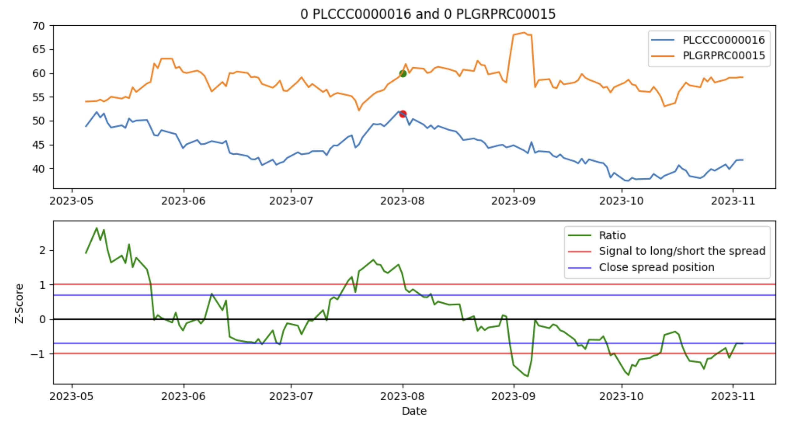
The program fetches current data couple of times a day, sees that current Z-Score ratio didn’t cross the safety zone between two blue lines, and so finally recommends to buy 0 CCC and 0 GRPRC. This graph (and all others for different pairs) gets sent to us via email.
We can decide that we want to enter a trade and type its details manually to a .csv file. They will be taken into account when the program suggests other decisions in the future.
Mock trading game
Everything was ready before the game has started - even the backtests were showing some functionality. Below is one of them, with (unintentionally) negative average return. But some occasional positive returns.
We entered the one-week mock trading game with enthusiasm, but were surprised to see the platform didn’t allow any sort of mechanism for short selling.
At first, I really thought there was nothing to be done and we should just all-in into the most volatile stock with the largest beta. Fortunately, a kind contest staff member noticed there could be some advantage taken of the inverse ETF.
So the majority of my code had to be rewritten. And there was only a small chance that the approximate short positions would be correlated enough with an ideal short position my backtests assumed.
Approximating shorting
Data
The entire previous logic stayed more or less the same. The core mechanism that was added was how we establish a short position.
The WIG20 Short ETF moves inversely to the WIG20 index. If WIG20 moves $15\%$ up, WIG20 Short moves $15\%$ down.
WIG20 consists of some 20 largest companies in Poland, chosen by a certain committee. Their inclusion is weighted by market capitalisation and some other factors.
We assumed constituents percenteges do not change. The reason was that the Warsaw Stock Exchange commitee adjusts the index around every 6 months, which is 2 times longer than the whole span of the game. So I assumed I don’t have to ask Mikołaj to write an entire module for fetching constituents data.
The Mechanism
The idea was pretty simple. Imagine the Inverse $\text{ABC-Short ETF}$ contains companies $A, B$ and $C$, respectively with percantages $10\%, 30\%, 60 \%$. If we want to short company $A$, we buy $10$ of $\text{ABC-Short ETF}$, $3$ stocks of company $B$ and $6$ stocks of company $C$. $10$ of $\text{ABC-Short ETF}$ would ensure a $-1$ position on $A$, $-3$ position on $B$ and $-6$ position on $C$. So we rebalance the position to be neutral on $B, C$ and arrive with the desired result.
The caveat is that the percentages in WIG20 are often so small we don’t have enough funds to have a great short approximation. So in reality the $\text{ABC-Short ETF}$ could be worth $\ $10 $ and the company $B$ could be worth $ $500 $ and you would have to have at least $500 + 10 \cdot ( 500 / (10 \cdot 30\%) ) = $ 2166.66 $ to be short on $A$ instead of just the cost of $A$.
Of course, there is some slippage of transactions costs, but I thought that this would be addressed after seeing the whole strategy in action (with the above Mechanism implemented.)
The Mechanism would return the best approximate position to short a given stock, or indicate if it wasn’t possible. It also returned the Pearson correlation coefficient of the approximate short position changes and the ideal short position changes. The strategy later parametrized the minimum acceptable Pearson for backtesting purposes (if Pearson is too low the short position on one of the stocks in the pair is too risky.)
In reality the Pearson coefficient for different pairs was about $0.6$.
Backtest results
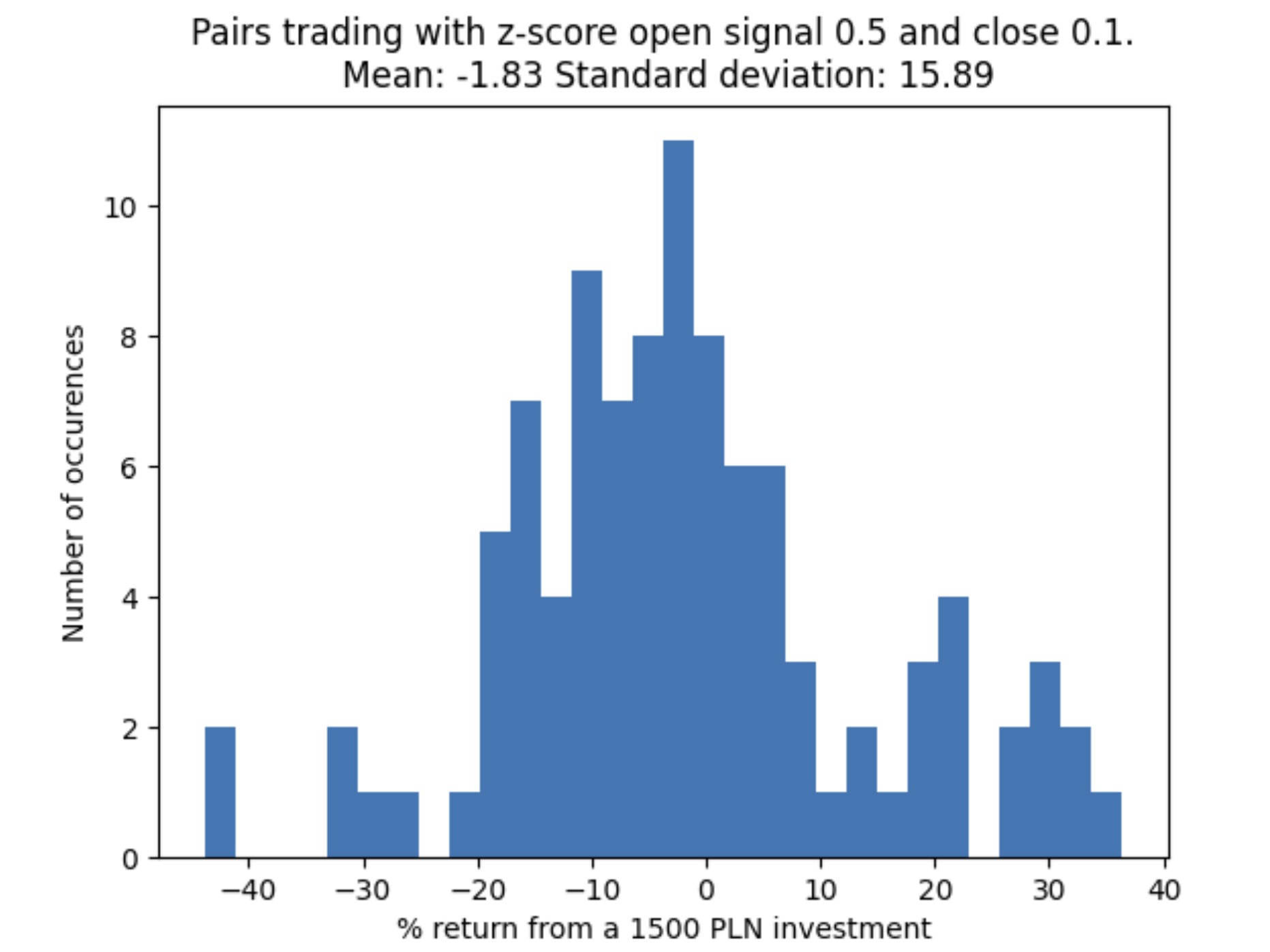
The backtests for the updated strategy simulated random 2 months snapshots at different pairs. Although the game spanned 3 months we wanted to be secure that some trades could have been exited fast enough - in addition, the time was running and I was a week late already.
The backtesting program had a couple of parameters: number of simulated samples, Z-Score close (how wide is the safety zone), Z-Score signal (how wide is the zone indicating when to short/long a spread), Z-Score lookback period (from how many days back do we calculate the mean and standard deviation of the ratio) and the minimum acceptable Pearson coefficient returned by above Mechanism.
I iterated over different combinations of these values and plotted all of the results at once, before inspecting what the optimal choice was.
.png)
These backtests were a nail in the coffin. There was not a sample time period and a parameters choice that resulted in positive profit.
Conclusions
Allocation remark
One mistake I realized long after the game was how we could have changed the value function $f(q_1, q_2)$ from the section “Trading with the pairs & system overview” to give more importance to the first summand - an allocation that doesn’t have the same (absolute) value of two positions on a pair is biased towards one of the stocks.
We could somehow fix this by parametrizing the function $f$ with a paramater $\alpha \in (0, 1)$ and backtesting to find its optimal value:
\[f(q_1, q_2, \alpha) = \alpha \cdot ( \frac{q_1 \cdot \text{price}_1}{q_2 \cdot \text{price}_2} - 1) ^ 2 + (1 - \alpha ) \cdot (\frac{q_1 \cdot \text{price}_1 + q_2 \cdot \text{price}_2}{\text{available funds}}) ^ 2\]Even more drastically, we could even map each $(q_1, q_2)$ to a pair of values $( ( \frac{q_1 \cdot \text{price}_1}{q_2 \cdot \text{price}_2} - 1) ^ 2, (\frac{q_1 \cdot \text{price}_1 + q_2 \cdot \text{price}_2}{\text{available funds}}) ^ 2)$ and sorting them lexicograhically (so by the first value - and if they are equal - by the second value).
But this is all guesswork and I don’t know if this has any science behind it.
Shorting Mechanism remark
I was happy that the my shorting approximation had a relatively high Pearson correlation of about $0.6$. I had a thought that this was a result of the low beta of each stock that was shorted and so the shorting approximation was essentially useless. But this seems like circular reasoning and I would need to think about it more.
Epilogue
Thinking that this paper about Non-Stationary Transformers was relatively new we run it on our data and did all-in on one of the stocks that had the highest expected returns. We held it for a week and sold it for minor profit.
Two weeks before the deadline we decided that we would have to dump all our money into one stock that had a low correlation with the whole market to gain any advantage in the ranking. We had an accidental $3\%$ return.
In the end, contest staff has decided to qualify all teams that showed any sign of activity, no matter its place in the ranking. So we qualified to the second round.